Show code cell content
# Install the necessary dependencies

import os
import sys
!{sys.executable} -m pip install --quiet pandas scikit-learn numpy matplotlib jupyterlab_myst ipython tensorflow_addons opencv-python requests
5. Diffusion Model#
5.1. Overview#
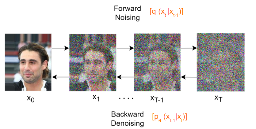
Diffusion model in deep learning is a type of generative model. The core idea of this model is to generate data by gradually adding noise. Specifically, diffusion models achieve data generation through two processes: diffusion process and inverse diffusion process.
Forward Diffusion Process: In this process, the model gradually adds noise to the data, making it increasingly random and unpredictable. Reverse Diffusion Process: This process attempts to gradually remove the added noise, gradually restoring the data to its original state.
By alternately applying these two processes, diffusion models can generate high-quality data samples.
5.2. Background#
Before we learn the diffusion model, we have to know some background knowledge in statistics. Perhaps you already have a good mastery of them, let’s review them together.
5.2.1. Expectation#
5.2.1.1. Definition#
In probability theory, expectation (also called expected value, mean, average) is a generalization of the weighted average.
\(E[X] = x_1 p_1 + x_2 p2 + ... +x_n p_n = \sum_{i=1}^n x_i p_1\)
where \(x_i\) and \(p_i\) are i-th a possible outcome and its probability, respectively.
5.2.1.2. Properties#
\(E[aX]=aE[X]\) where a is a constant value.
\(E[X+b]=E[X]+b\) where b is a constant value.
\(E[X+Y]=E[X]+E[Y]\).
5.2.2. Variance#
Variance is a measure of dispersion, meaning it is a measure of how far a set of numbers is spread out from their average value.
5.2.2.1. Definition#
The variance of a random variable \(X\) is the expected value of the squared deviation from the expectation of \(X\).
5.2.2.2. Properties#
\(Var[X]=E[X^2]−E[X]^2\).
\(Var[aX]=a^2 Var[X]\) where a is a constant value.
\(Var[X+b]=Var[X]\) where b is a constant value.
\(Var[X+Y]=Var[X]+Var[Y]\).
5.2.3. Re-parameterization trick#
When we sample data from a probability distribution, backpropagation the gradient is not possible because it is a stochastic process. To make it trainable, the re-parameterization trick is useful.
Let us assume that \(z\) is sampled data from a gaussian distribution which the mean is \(\mu\) and the variance is \(\sigma^2\). Then, the mean and variance of \(z\) would be \(\mu\) and \(\sigma^2\). Therefore, \(z\) can be written as follows.
\(z = N(\mu, \sigma^2 I) = \mu + \sigma \odot \epsilon\), where \(\epsilon \thicksim N(0, I)\)
where \(\odot\) refers to element-wise product.
The mean and variance of \(z\) correspond to \(\mu\) and \(\sigma^2\), respectively.
5.2.3.1. Mean (Expectation)#
\(E[z] = E[\mu+\sigma \odot \epsilon] = E[\mu] + \sigma E[\epsilon] = \mu\)
The expectation of \(\epsilon\) is 0 by definition.
5.2.3.2. Variance#
\(Var[z] = Var[\mu + \sigma \odot \epsilon] = Var[\sigma \odot \epsilon] = \sigma^2 Var[\epsilon] = \sigma^2\)
The variance of \epsilon is 1 by definition.
5.2.4. KL Divergence#
In mathematical statistics, the Kullback–Leibler divergence (relative entropy), is a type of statistical distance.
5.2.4.1. Definition#
Discrete probability distribution
\(D_{KL}(P||Q) = \sum_{x \in X} P(x) log \frac{P(x)}{Q(x)}\),where \(P\) and \(Q\) are discrete probability distributions.
Continuous probability distribution
\(D_{KL} (P||Q) = \int _{− \infty}^{\infty} p(x) log \frac{p(x)}{q(x)}dx\), where \(p\) and \(q\) denote the probability densities of \(P\) and \(Q\).
5.2.4.2. Jensen’s inequality#
In mathematics, Jensen’s inequality relates the value of a convex (or concave) function of an integral to the integral of the function.
Convex function: \(f(E[X]) \leqq E[f(X)]\);
Concave function: \(f(E[X]) \geqq E[f(X)]\).
5.2.4.3. Properties of KL Divergence#
KL Divergence is always non-negative;
The cross-entropy is always larger than the entropy;
Two univariate normal distributions \(P\) and \(Q\) are simplified to \(D_{KL}(P||Q) = log \frac{\sigma_q}{\sigma_p} + \frac{\sigma^2_p + (\mu_p − \mu_q)^2}{2\sigma^2_q} − \frac{1}{2}\).
5.2.5. Evidence lower bound (ELBO)#
In variational Bayesian methods, the evidence lower bound (often abbreviated ELBO) is a useful lower bound on the log-likelihood of some observed data.
5.2.5.1. Definition#
\(ELBO := E_{z∼q_{\phi}}[log \frac{pθ(x,z)}{q_{\phi}(z)}]\)
where \(p_{\theta}(x, z)\) is joint distribution of \(x\) and \(z\). \(\theta\) and \(\phi\) are parameters.
ELBO is used to obtain the lower bound of the evidence (or log evidence). The evidence is the likelihood function evaluated at a fixed \(\theta\).
\(evidence := log p_{\theta}(x)\)
5.2.5.2. Properties#
The evidence is always larger than ELBO;
KL Divergence between \(p_{\theta}(z|x)\) and \(q_{\phi}(z)\) equals \(evidence−ELBO\).
6. Forward and Reverse Process#
Diffusion models transform data into Gaussian noise (latent vector) and then restore it. The former is called the forward process, and the latter is called the reverse process.
6.1. Forward Diffusion Process#
In the forward process, we add a gaussian noise to the data step by step (usually hundreds of steps).
The transform of an individual step is defined as follows. \(x_t = q(x_t|x_{t−1}) = N(x_t, \sqrt{1−\beta_t}x_{t−1}, \beta_t I)\)
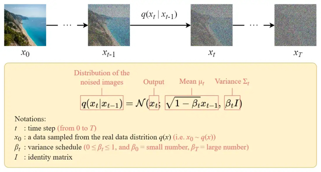
The forward diffusion process progressively adds Gaussian noise to the input image \(x_0\) over \(T\) steps, producing a series of noisy image samples \(x_1, \ldots, x_T\).
As \(T \rightarrow \infty\), the final result will converge to an image fully corrupted by noise, akin to sampling from an isotropic Gaussian distribution.
The inefficiency of Pythonic loops, particularly with large timestamps, can cause significant slowdowns. To address this, we employ a reparameterization trick, which uses an approximation method to generate noise at specific timestamps, avoiding the need for explicit iteration.
\(\alpha_t := 1 - \beta_t\), \(\bar{\alpha}_t := \prod_{s=1}^{t} \alpha_s\), \(q(x_t | x_0) = \mathcal{N}\left( x_t; \sqrt{\bar{\alpha}_t} x_0, (1 - \bar{\alpha}_t) I \right)\)
We’ve isolated the variance schedule and calculated the cumulative product of this variable \(α_t\). This equation allows us to directly sample the noisy image at any time step using just the original image \(( x_0 )\).
6.2. Reverse Diffusion Process#
In the reverse process, we restore image from a gaussian noise (a latent vector). If \(\beta_t\) is small enough, the reverse \(q(x_{t-1}|x_t)\) will also be gaussian. It is noteworthy that the reverse process is tractable when conditioned on \(x_0\).
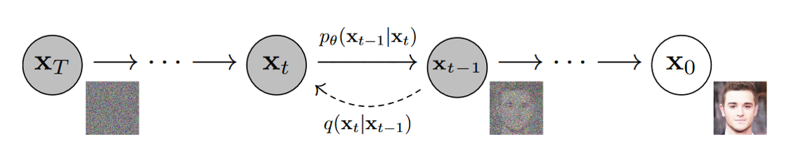
The forward process is different; we cannot use \(q(x_{t-1}|x_t)\) to reverse the noise because it is difficult (or impossible) to compute. Therefore, we need to train a neural network \(p_θ(xₜ₋₁|xₜ)\) to approximate \(q(x_{t-1}|x_t)\).
\(p_{\theta}(x_{t-1}|x_{t}) := \mathcal{N}(x_{t-1}; \mu(x_{t}, t), \Sigma_{\theta}(x_{t}, t))\)
\(p_{\theta}(x_{0:T}) = p_{\theta}(x_{T}) \prod_{t=1}^{T} p_{\theta}(x_{t-1}|x_{t})\)
\(p_{\theta}(x_{0}) := \int p_{\theta}(x_{0:T}) dx_{1:T}\)
6.2.1. Loss Function#
In a diffusion model, the goal of the reverse diffusion process is to infer the noise-free original image that generated the observed noisy image. To achieve this, we train a neural network to approximate the inverse of the noise process. The training of this neural network is accomplished by minimizing a loss function.
First,We define loss function using negative log likelihood & ELBO:
Then,chenge to tractable form:
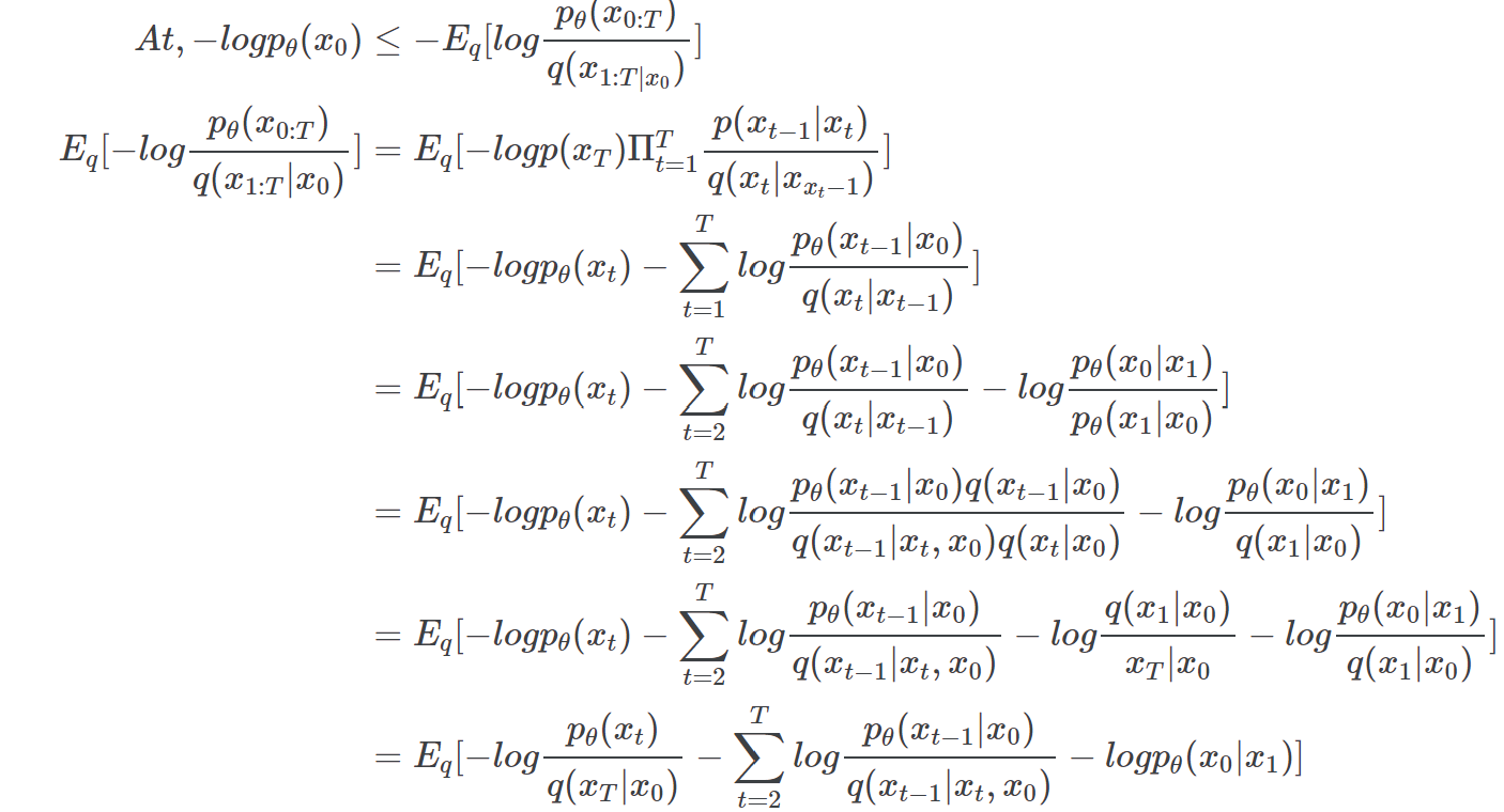
Finally,simplify training objective:
We will use \(D_{KL}(q(x_{t-1} | x_t, x_0) || p_{\theta}(x_{t-1} | x_t) )\) for simplifying the loss function. In the paper, the author trained the model using this part as a training objective.
So, our challenge has been narrowed down to training the two distributions \( q(x_{t-1} | x_t, x_0) \) and \( p_{\theta}(x_{t-1} | x_t) \) as equally as possible.
Final Loss: $\( \begin{aligned} E_{x_0, \epsilon}[ || \epsilon - \epsilon_{\theta}(\sqrt{\hat{\alpha}_t}x_0 + \sqrt{1 - \hat{\alpha}_t} \epsilon, t) ||^2 ] \end{aligned} \)$
6.2.2. Noise schedule#
In diffusion models, the noise schedule define the methodology for iteratively adding noise to an image or for updating a sample based on model outputs. I’ll introduce two type of schedules which are linear schedule and cosine schedule. The linear and cosine schedule were introduced by Denoising Diffusion Probabilistic Models and Improved Denoising Diffusion Probabilistic Models, respectively.
6.2.2.1. Linear schedule#
The linear schedule is a simple noise scheduling method that controls the size of noise in each diffusion step linearly. Specifically, the linear schedule gradually increases the noise level at a fixed rate in each diffusion step until it reaches the maximum noise level.
In the linear schedule, \(\beta_t\) changes linearly.
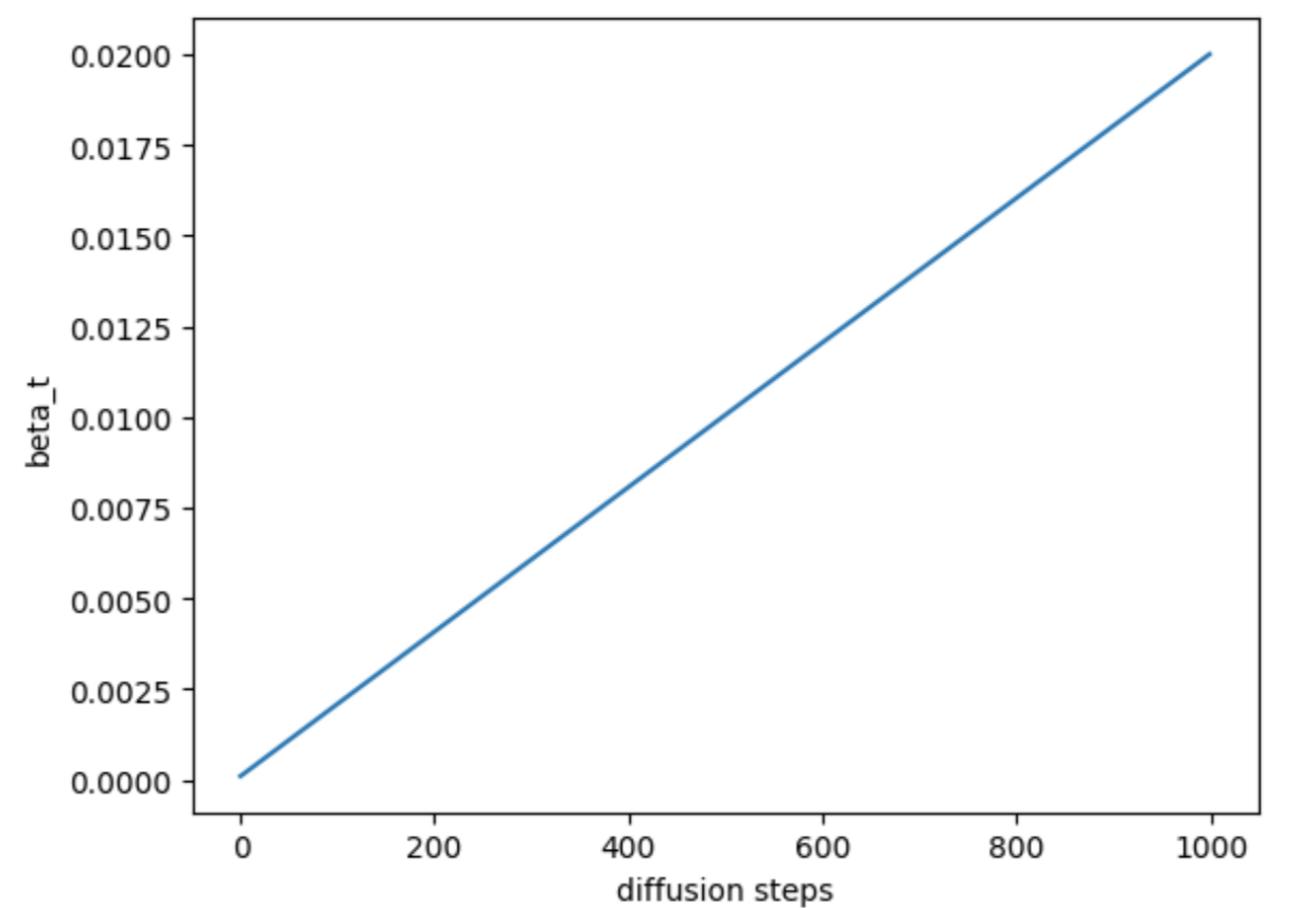
Illustration of linear schedule
6.2.2.2. Cosine schedule#
The cosine schedule is a noise scheduling method based on the cosine function, which adjusts the noise level during the diffusion process. The key idea of the cosine schedule is to start with a high noise level in the early iterations, gradually decrease the noise level during the iteration process, and finally converge to a lower level.
Alex Nichol and Prafulla Dhariwal proposed the cosine schedule to prevent an image from turning into noise too quickly. They construct a different noise schedule in terms of \(\overline{\alpha_t}\).
\(\overline{\alpha_t} = \frac{f(t)}{f(0)}\), \(f(t) = cos(\frac{\frac{t}{T} + s}{1+s} \frac{\pi}{2})^2\). By definition, the \(\beta_t\) equals \(1 - \frac{\overline{\alpha_t}}{\overline{\alpha_{t-1}}}\).
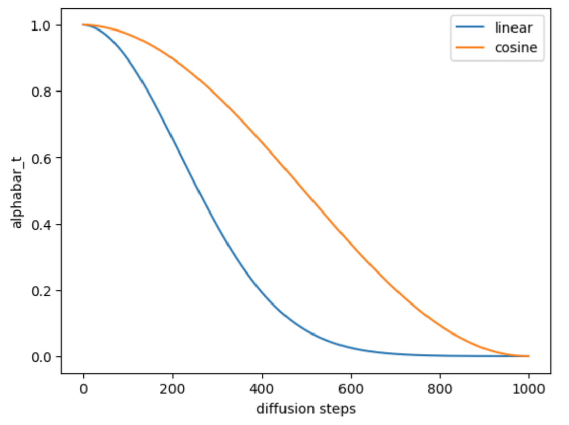
Illustration of cosine schedule
6.3. Code#
6.3.1. Import Libraries#
import tensorflow as tf
import numpy as np
import cv2
import time
import requests
import zipfile
import io
import matplotlib.pyplot as plt
import matplotlib.animation as animation
from tensorflow.keras.models import Model
from tensorflow.keras.layers import Layer
from tensorflow.keras.layers import (Reshape, Conv2DTranspose, Add, Conv2D, MaxPool2D, Dense,
                                     Flatten, Input, BatchNormalization, Input, MultiHeadAttention)
from tensorflow.keras.optimizers import Adam
import tensorflow_addons as tfa
BATCH_SIZE = 32
TIME_STEPS = 1000
IM_SHAPE = (32,32,3)
N_HEADS = 8
ATTN_DIM = 256
N_GROUPS = 8
N_RESNETS = 2
LEARNING_RATE = 2e-4
EPOCHS = 10
FACTOR = 2
6.3.2. Data Loading#
The dataset can be downloaded from here.
url = 'https://static-1300131294.cos.ap-shanghai.myqcloud.com/data/deep-learning/diffusion-model/archive.zip'

r = requests.get(url)
with zipfile.ZipFile(io.BytesIO(r.content), 'r') as zip_ref:
    zip_ref.extractall('./')
ds_train = tf.keras.preprocessing.image_dataset_from_directory(
    "t/celebA", label_mode=None, image_size=(IM_SHAPE[0], IM_SHAPE[1]), batch_size=BATCH_SIZE)
6.3.3. Data Preprocessing#
def preprocess(image):
    return tf.cast(image, tf.float32) / 127.5 - 1.0
6.3.4. Data Augmentation#
def augmentation(image):
    return tf.image.random_flip_left_right(image)
6.3.5. Data#
train_dataset = (
    ds_train
    .map(preprocess)
    .map(augmentation)
    .unbatch()
    .shuffle(buffer_size = 1024, reshuffle_each_iteration = True)
    .batch(BATCH_SIZE,drop_remainder=True)
    .prefetch(tf.data.AUTOTUNE))
6.3.6. Linear schedule-beta#
def linear_beta_schedule(timesteps):
    beta_start = 0.0001
    beta_end = 0.02
    return tf.linspace(beta_start, beta_end, timesteps)
betas = linear_beta_schedule(TIME_STEPS)
print(betas)
alphas = 1. - betas
alphas_cumprod = tf.math.cumprod(alphas, axis=0)
sqrt_alphas_cumprod = tf.math.sqrt(alphas_cumprod)
sqrt_one_minus_alphas_cumprod = tf.math.sqrt(1. - alphas_cumprod)
def extract(a, t, x_shape):
    b, *_ = t.shape
    out = tf.gather(a,t)
    output = tf.reshape(out, (b,*((1,) * (len(x_shape) - 1))))
    return output

def q_sample(x_start, t, noise):

    sqrt_alphas_cumprod_t = extract(sqrt_alphas_cumprod, t, x_start.shape)
    sqrt_one_minus_alphas_cumprod_t = extract(sqrt_one_minus_alphas_cumprod, t, x_start.shape)

    out_sample = sqrt_alphas_cumprod_t * x_start + sqrt_one_minus_alphas_cumprod_t * noise### x_start=x_0, noise = z
    return out_sample
class PositionalEmbeddings(tf.keras.layers.Layer):

    def __init__(self, dim):
        super().__init__()
        self.embedding_dim = dim

    def get_timestep_embedding(self, timesteps, embedding_dim: int):
        """
        From Fairseq.
        Build sinusoidal embeddings.
        This matches the implementation in tensor2tensor, but differs slightly
        from the description in Section 3.5 of "Attention Is All You Need".
        """
        half_dim = self.embedding_dim // 2
        emb = tf.math.log(10000.) / (half_dim - 1)
        emb = tf.exp(tf.range(half_dim, dtype=tf.float32) * -emb)
        emb = tf.cast(timesteps, dtype = tf.float32)[:, None] * emb[None, :]
        emb = tf.concat([tf.sin(emb), tf.cos(emb)], axis=1)
        if embedding_dim % 2 == 1:
            emb = tf.pad(emb, [[0, 0], [0, 1]])
        return emb

    def call(self, time):
        return self.get_timestep_embedding(time, self.embedding_dim)
def res_block(x,filters,n_groups,temb):
    previous = x
    x = Conv2D(filters, 3, padding="same",)(x) ### Convolution layer with padding same, so that the resolution remains the same

    ### temb represents the time embedding.
    ### It is passed into the silu activation function and a Dense Layer(Which can change the the embedding dimension )
    ### We also reshape the time embedding to match the output of 2d convnets.
    x += Dense(filters)(tf.nn.silu(temb))[:,None,None,:]

    ### Group Normalization is used.
    x = tf.nn.silu(tfa.layers.GroupNormalization(n_groups, axis = -1)(x))
    x = Conv2D(filters, 3, padding="same",)(x)

    # Project residual
    residual = Conv2D(filters, 1,padding="same",)(previous)
    x = tf.keras.layers.add([x, residual])  # Add back residual
    return x

def get_model(im_shape=(64,64,3),n_resnets=2,n_groups=8,attn_dim=32,n_heads=4,):
    input_1 = Input(shape=im_shape)### image input
    input_2 = Input(shape=())### time input
    t_dim = im_shape[0]*16

    # Entry block
    x = Conv2D(32, 3, padding="same")(input_1)
    temb = PositionalEmbeddings(t_dim)(input_2)### Create embeddings from the time input_2
    temb = Dense(t_dim)(tf.nn.gelu(Dense(t_dim)(temb)))### pass the embedding into the gelu activation function

    hs = [x]### variable used for storing each resolution level output, in the downward path, to be concatenated to the inputs of the upward path.

    ### Downward Path
    for filters in [32, 64, 128, 256]:### for every resolution level (32,64,128,256), represent the depth they map to resolutions of (32,16,8,4)
        for _ in range(n_resnets):### we go through each resnet block per resolution level
            x = res_block(x,filters,n_groups,temb)### resblock
            ### if the resolution=16 (coinciding with a depth=64), we make the resnet output features attend to each other.
            ### Note how the attention axes = (1,2). This corresponds to the height and width dimensions.
            ### Feel free to Check the documentation out :) https://www.tensorflow.org/api_docs/python/tf/keras/layers/MultiHeadAttention.
            ### query = key = value = x.
            ### We again use Group Normalization.
            if filters == 64:
                x = tfa.layers.GroupNormalization(groups=n_groups, axis = -1)(
                    MultiHeadAttention(num_heads=n_heads, key_dim=attn_dim, attention_axes=(1,2), )(query = x, value = x))
        hs.append(x)### append the output features to hs
        x = tf.keras.layers.MaxPooling2D(3, strides=2, padding="same")(x)### Downsampling in order to move to the next resolution level


    ### Bottleneck
    x = res_block(x,256,n_groups,temb)
    x = tfa.layers.GroupNormalization(groups=n_groups, axis = -1)(
      MultiHeadAttention(num_heads=n_heads, key_dim=attn_dim, attention_axes=(1,2), )(query = x, value = x))
    x = res_block(x,256,n_groups,temb)


    ### Upward path
    for filters in [256, 128, 64,32]:
        ### we resize x, to match with the shape of feature outputs (hs) in the downward path
        x = tf.image.resize_with_pad(x,hs[-1].shape[1],hs[-1].shape[2])
        x = tf.concat([x,hs.pop()], axis=-1)

        for _ in range(n_resnets):
            x = res_block(x,filters,n_groups,temb)

            if filters == 64:
                x = tfa.layers.GroupNormalization(groups=n_groups, axis = -1)(
                  MultiHeadAttention(num_heads=n_heads, key_dim=attn_dim, attention_axes=(1,2), )(query = x, value = x))

        if filters != 32:
            x = Conv2DTranspose(filters, 3, strides = (2,2),)(x)### Upsampling

    x = res_block(x,32,n_groups,temb)
    outputs = Conv2D(3, 3, padding="same", )(x)

    # Define the model
    model = Model([input_1,input_2], outputs,name='unet')
    return model

model= get_model(im_shape=IM_SHAPE,n_resnets=N_RESNETS,n_groups=N_GROUPS,attn_dim=ATTN_DIM,n_heads=N_HEADS,)
model.summary()
class LRSchedule(tf.keras.optimizers.schedules.LearningRateSchedule):

    def __init__(self, init_lr):
        self.init_lr = init_lr

    def __call__(self, step):
        return self.init_lr*(100000/(step+100000))

OPTIMIZER = Adam(learning_rate=LRSchedule(1e-4))

def custom_loss(denoise_model, x_start, t, noise=None):
    ### Our custom loss function takes in the predicted noise and compares (using the Huber Loss) it with the actual noise
    ### Huber Loss with a default value for delta as 1.0 Check out the documentation: https://www.tensorflow.org/api_docs/python/tf/keras/losses/Huber
    h = tf.keras.losses.Huber()
    noise = tf.random.normal(x_start.shape,mean=0,stddev=1)### noise=epsilon=z
    x_noisy = q_sample(x_start,t,noise)### x_t using the q_sample method
    predicted_noise = denoise_model([x_noisy, t])### model takes in the x_t and t and outputs noise
    return h(noise,predicted_noise)

### custom training block
### You can use tf.function to make graphs out of your programs. It is a transformation tool that creates Python-independent dataflow graphs
### out of your Python code. This will help you create performant and portable models.
@tf.function
def training_block(x_batch):
    with tf.GradientTape() as recorder:
        ### for every element in the batch, we generate t randomly
        t = tf.random.uniform((BATCH_SIZE,),minval=0,maxval=TIME_STEPS,dtype=tf.int32)
        loss = custom_loss(model,x_batch,t)

    partial_derivatives = recorder.gradient(loss, model.trainable_weights)
    OPTIMIZER.apply_gradients(zip(partial_derivatives, model.trainable_weights))### gradient descent
    return loss

def neuralearn(EPOCHS):
    for epoch in range(EPOCHS):
        init_time = time.time()
        losses = []
        for step, x_batch in enumerate(train_dataset):
            loss = training_block(x_batch)
            losses.append(loss)

        print(str(epoch+1)+"/"+str(EPOCHS)+": Training Loss----->", sum(losses)/len(losses))
        print('Time Elapsed: ---> '+str(time.time()-init_time)+' s')

    print("Training Complete!!!!")

neuralearn(EPOCHS)
sqrt_recip_alphas = tf.math.sqrt(1.0 / alphas)
alphas_cumprod_prev = tf.concat([tf.ones((1,)),alphas_cumprod[:-1]],axis = 0)### alpha_t-1_bar = alphas_cumprod_prev

posterior_variance = betas * (1. - alphas_cumprod_prev) / (1. - alphas_cumprod)

def p_sample(model, x, t, t_index):

    betas_t = extract(betas, t, x.shape)### betas_t = 1-alphas_t
    sqrt_one_minus_alphas_cumprod_t = extract(sqrt_one_minus_alphas_cumprod, t, x.shape)### square root of 1-alpha_t_bar
    sqrt_recip_alphas_t = extract(sqrt_recip_alphas, t, x.shape)### 1/square root of alpha_t

    model_mean = sqrt_recip_alphas_t * (x - betas_t * model([x, t]) / sqrt_one_minus_alphas_cumprod_t)### equation 4 of algorithm 2 above

    if t_index == 0:
        return model_mean
    else:
        posterior_variance_t = extract(posterior_variance, t, x.shape)### sigma_t
        noise = tf.random.normal(x.shape)
        return model_mean + tf.math.sqrt(posterior_variance_t) * noise

imgs = []
img = tf.random.normal((64,IM_SHAPE[0],IM_SHAPE[1],IM_SHAPE[2]))
for i in reversed(range(0, TIME_STEPS)):### we go backwards from t = 1000 to t = 0
    print(i)
    img = p_sample(model,img,tf.fill((1,),i,), i)
    imgs.append(img)

plt.figure(figsize = (16,16))

for i in range(32):
    ax = plt.subplot(4,8, i+1)
    plt.imshow(np.array(imgs[999])[i])
    plt.axis("off")
random_index = 0

fig = plt.figure()
ims = []
for i in range(TIME_STEPS):
    im = plt.imshow(np.array(imgs[i])[random_index], animated=True)
    ims.append([im])
    ims.append([im])

animate = animation.ArtistAnimation(fig, ims, interval=5, blit=True, repeat_delay=1000)
animate.save('diffusion.gif')
plt.show()
6.4. Your turn! 🚀#
Assignment - Denoising difussion model
6.5. Acknowledgments#
Thanks to Kwangnam Yu for creating the open-source project diffusion_models_tutorial and kaggle for creating the open-source courses Denoising Diffusion Models with TensorFlowExploring Diffusion Models with JAXDenoising Diffusion Probabilistic Model with TF. They inspire the majority of the content in this chapter.